Bayes vs. the Invaders! Part One: The 37th Parallel

Introduction

From our earlier studies of UFO sightings, a recurring question has been the extent to which the frequency of sightings of inexplicable otherworldly phenomena depends on the population of an area. Intuitively: where there are more people to catch a glimpse of the unknown, there will be more reports of alien visitors.

Is this hypothesis, however, true? Do UFO sightings closely follow population or are there other, less comforting, factors at work?

In this short series of posts, we will build a statistical model of UFO sightings in the United States, based on data previously scraped from the National UFO Reporting Centre and see how well we can predict the rate of UFO sightings based on state population.

This series of posts is part tutorial and part exploration of a set of modelling tools and techniques. Specifically, we will use Generalized Linear Models (GLMs), Bayesian inference, and the Stan probabilistic programming language to unveil the relationship between unsuspecting populations of US states and the dread sightings of extraterrestrial truth that they experience.

Data

As mentioned, we will rely on data from NUFORC for extraterrestrial sightings.

For population data, we can rely on the the FRED database for historical US state-level census data. The combination of these datasets provides us with a count of UFO sightings per year for each state, and the population of that state in that year.

The downloading and scraping code is included here:

Show scraping code.

ZSH script to download via `curl`
[code language=”bash”] #!/bin/zsh
# Download US state-level population datasets from FRED
# State series names are stored in the file ‘series_names’ (downloaded from fred.stlouisfed.org)
# <https: fred.stlouisfed.org="" release?rid="118">
#
# The per-series requests is included below.</https:>

export IFS=$’\n’

# Download
for state_series in $(cat series_names); do

curl -o "output/$state_series.csv" "https://fred.stlouisfed.org/graph/fredgraph.csv?bgcolor=%23e1e9f0&amp;chart_type=line&amp;drp=0&amp;fo=open%20sans&amp;graph_bgcolor=%23ffffff&amp;height=450&amp;mode=fred&amp;recession_bars=on&amp;txtcolor=%23444444&amp;ts=12&amp;tts=12&amp;width=1168&amp;nt=0&amp;thu=0&amp;trc=0&amp;show_legend=yes&amp;show_axis_titles=yes&amp;show_tooltip=yes&amp;id=$state_series&amp;scale=left&amp;cosd=1900-01-01&amp;coed=2018-01-01&amp;line_color=%234572a7&amp;link_values=false&amp;line_style=solid&amp;mark_type=none&amp;mw=3&amp;lw=2&amp;ost=-99999&amp;oet=99999&amp;mma=0&amp;fml=a&amp;fq=Annual&amp;fam=avg&amp;fgst=lin&amp;fgsnd=2009-06-01&amp;line_index=1&amp;transformation=lin&amp;vintage_date=2019-03-04&amp;revision_date=2019-03-04&amp;nd=1900-01-01"

done
[/code]

Necessary ‘series_names’ file:
[code language=”text”] WAPOP
GAPOP
CAPOP
MOPOP
DSPOP
ILPOP
TXPOP
NYPOP
FLPOP
ALPOP
COPOP
WIPOP
AZPOP
MIPOP
NCPOP
MAPOP
CTPOP
LAPOP
OHPOP
AKPOP
TNPOP
MNPOP
NJPOP
NMPOP
ARPOP
MDPOP
PAPOP
NVPOP
IAPOP
ORPOP
T5POP
DCPOP
HIPOP
NDPOP
KYPOP
VAPOP
IDPOP
KSPOP
INPOP
WVPOP
RIPOP
SCPOP
MSPOP
DEPOP
MTPOP
MEPOP
NEPOP
OKPOP
WYPOP
UTPOP
NHPOP
VTPOP
SDPOP
[/code]

R code to combine data into tidy format
[code language=”r”] library( tidyverse )

# Read all CSV files
census_files <- list.files( "output", full.names=TRUE )

# Join all data into a single table
census_data <-
census_files %>%
map( read_csv ) %>% # Read each file, forming a list with an element for each
reduce( full_join, by="DATE" ) %>% # Reduce (left to right) running a full join
dplyr::arrange( DATE ) %>% # Sort by date
gather( key="state", value="population", -DATE ) %>% # Gather to long format
transmute( date=DATE, state=str_replace( state, "POP", "" ), population ) # Rename and tidy variables and names

# Output to an .rds
saveRDS( census_data, "data/annual_population.rds" )

[/code]

For ease, we will treat each year’s count of sightings as independent from the previous year’s — we do not make an assumption that the number of sightings in each year is based on the number of sightings in the previous year, but is rather due to the unknowable schemes of alien minds. (If extraterrestrials visitors were colonising areas in secrecy rather than making sporadic visits, and thus being seen repeatedly, we might not want to make such a bold assumption.) Each annual count will be treated as an individual, independent data point relating population to count, with each observation tagged by state.

For simplicity, particularly in building later models, we will restrict ourselves to sightings post 1990, roughly reflecting a period in which the NUFORC data sees a significant increase in reporting and thus relies less on historical reports. (NUFORC’s phone hotline has existed since 1974, and its web form since 1998.)

An Awful Simplicity

To begin, we start with the most basic form of model: a simple linear relationship between the count of sightings and the population of the state at that time. If sightings were purely dependent on population, it might be reasonable to assume that such a model would fit the data fairly well.

This relationship can be plotted with relative ease using the geom_smooth() function of ggplot2 in R. For opening our eyes to the awful truth contained in the data, this is a useful first step.
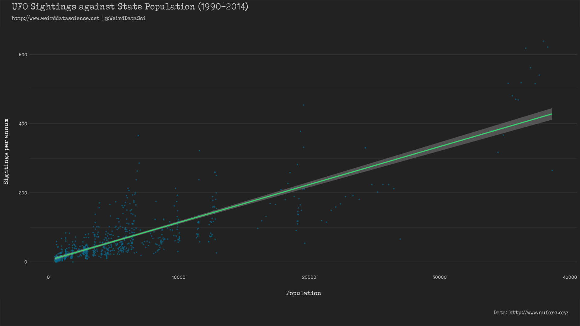
Regression of UFO sightings against population.
Global linear regression of UFO sightings against population. (PDF Version)

While this graph does seem to support the argument that sightings increase with population in general, a closer inspection shows that the individual data points are clearly clustered. If we highlight the location of each data point, colouring points by US state, this becomes clearer:
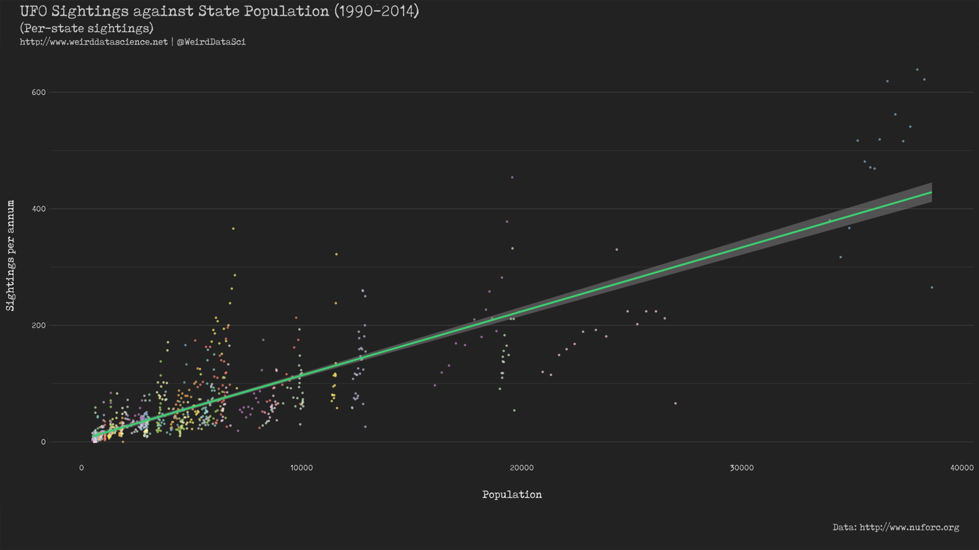
Global linear regression of UFO sightings against population with per-state colours.
Global linear regression of UFO sightings against population with per-state colours. (PDF Version)

This strongly suggests that, in preference to the simple linear model across all sightings, we might instead fit a linear model individually to each state:
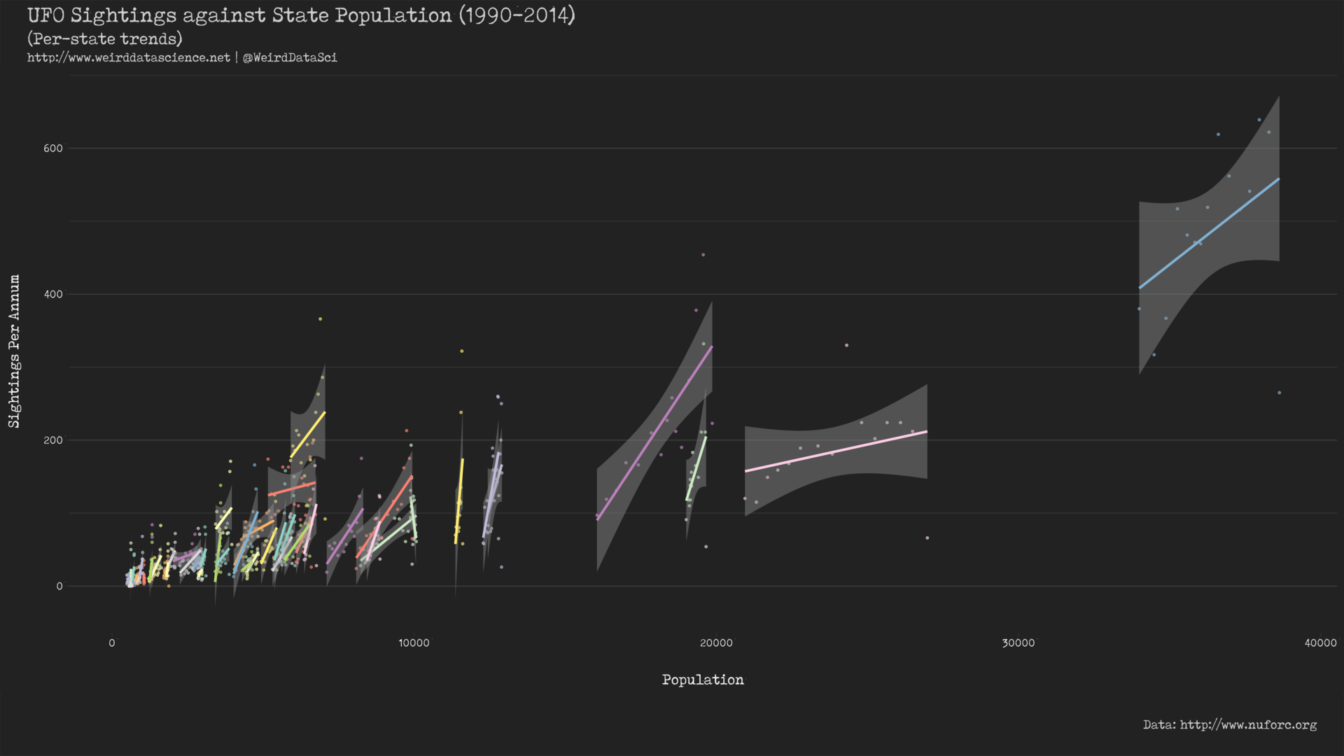
Per-state linear regression of UFO sightings against population,
Per-state linear regression of UFO sightings against population. (PDF Version)

The code to produce the above graphs from the NUFORC and FRED data is given below:

Show data preparation and visualization code.

Prepare and combine datasets:
[code language=”r”] library( tidyverse )
library( magrittr )
library( lubridate )

# Prepare data for model fitting (and plotting)

# Load US population and UFO datasets
ufo <- read_csv( "data/ufo_spatial.csv" )
census <- readRDS( "data/annual_population.rds" )

# Process UFO data to per-state counts per year.
# Drop Puerto Rico as we don’t have census data. (Also, very few sightings — 33 in dataset.)
ufo_state_annual <-
ufo %>%
# US only
filter( country == "us" ) %>%
# Apologies to Puerto Rico.
filter( state != "pr" ) %>%
# Convert date to year, drop all other variables except state.
transmute( date = year( as.POSIXct( datetime, format="%m/%d/%Y %H:%M" ) ), state=str_to_upper( state ) ) %>%
# Group by year
group_by( date, state ) %>%
# Sum sightings
summarize( count = n() )

# Process census suitable for joining with UFO sightings.
# Drop "DS" state entry — ("Department of State"?)
census <-
census %>%
filter( state != "DS" ) %>%
mutate( date=year( date ) )

# Join datasets
ufo_population_sightings <-
full_join( ufo_state_annual, census )

# Missing data implies zero sightings.
# Restrict to post-1990 to avoid a high proportion of very small numbers of
# sightings.
ufo_population_sightings <-
ufo_population_sightings %>%
mutate( count = replace_na( count, 0 ) ) %>%
filter( !is.na( population ) ) %>%
filter( date >= 1990 ) %>%
filter( date <= 2014 )

saveRDS( ufo_population_sightings, "work/ufo_population_sightings.rds" )
[/code]

Fit linear trend in data via geom_smooth() using a linear model.
[code language=”r”] library( tidyverse )
library( magrittr )
library( lubridate )

library( ggplot2 )
library( showtext )
library( RColorBrewer )

library( cowplot )

# Load UFO data
ufo_population_sightings <-
readRDS("work/ufo_population_sightings.rds")

# UFO reporting font
font_add( "main_font", "/usr/share/fonts/TTF/weird/Tox Typewriter.ttf")
showtext_auto()

# Combined plot ignoring states.
ufo_pop_plot <-
ggplot( ufo_population_sightings, aes( x=population, y=count ) ) +
geom_point( colour="#0b6788", size=0.6, alpha=0.8 ) +
geom_smooth( method="lm", colour="#3cd070" ) + # UFO green
xlab( "Population" ) +
ylab( "Sightings per annum" ) +
theme_weird() +
theme(
axis.title.y = element_text( angle=90 )
)

# Construct full plot, with title and backdrop.
title <-
ggdraw() +
draw_label("UFO Sightings against State Population (1990-2014)", fontfamily="main_font", colour = "#cccccc", size=20, hjust=0, vjust=1, x=0.02, y=0.88) +
draw_label("http://www.weirddatascience.net | @WeirdDataSci", fontfamily="main_font", colour = "#cccccc", size=12, hjust=0, vjust=1, x=0.02, y=0.40)

data_label <- ggdraw() +
draw_label("Data: http://www.nuforc.org", fontfamily="main_font", colour = "#cccccc", size=12, hjust=1, x=0.98 )

ufo_pop_titled <-
plot_grid(title, ufo_pop_plot, data_label, ncol=1, rel_heights=c(0.1, 1, 0.1)) +
theme(
panel.background = element_rect(fill = "#222222", colour = "#222222"),
plot.background = element_rect(fill = "#222222", colour = "#222222"),
)

save_plot("output/lm_ufo_population_sightings-combined.pdf",
ufo_pop_titled,
base_width = 16,
base_height = 9,
base_aspect_ratio = 1.78 )

# Combined plot colouring states.
ufo_pop_plot_states <-
ggplot( ufo_population_sightings, aes( x=population, y=count ) ) +
geom_point( aes( colour=state ), size=0.6, alpha=0.8 ) +
geom_smooth( method="lm", colour="#3cd070" ) + # UFO green
xlab( "Population" ) +
ylab( "Sightings per annum" ) +
scale_colour_manual( values=rep( brewer.pal( name="Set3", n=12 ), times=5 ) ) +
theme_weird() +
theme(
axis.title.y = element_text( angle=90 ),
legend.position="none"
)

# Construct full plot, with title and backdrop.
title <-
ggdraw() +
draw_label("UFO Sightings against State Population (1990-2014)", fontfamily="main_font", colour = "#cccccc", size=20, hjust=0, vjust=1, x=0.02, y=0.88) +
draw_label("(Per-state sightings)", fontfamily="main_font", colour = "#cccccc", size=16, hjust=0, vjust=1, x=0.02, y=0.48) +
draw_label("http://www.weirddatascience.net | @WeirdDataSci", fontfamily="main_font", colour = "#cccccc", size=12, hjust=0, vjust=1, x=0.02, y=0.16)

data_label <- ggdraw() +
draw_label("Data: http://www.nuforc.org", fontfamily="main_font", colour = "#cccccc", size=12, hjust=1, x=0.98 )

ufo_pop_states_titled <-
plot_grid(title, ufo_pop_plot_states, data_label, ncol=1, rel_heights=c(0.1, 1, 0.1)) +
theme(
panel.background = element_rect(fill = "#222222", colour = "#222222"),
plot.background = element_rect(fill = "#222222", colour = "#222222"),
)

save_plot("output/lm_ufo_population_sightings-state.pdf",
ufo_pop_states_titled,
base_width = 16,
base_height = 9,
base_aspect_ratio = 1.78 )

# Combined plot colouring states with per-state trend lines.
ufo_pop_plot_states_trends <-
ggplot( ufo_population_sightings, aes( x=population, y=count ) ) +
geom_point( aes( colour=state ), size=0.6, alpha=0.8 ) +
geom_smooth( method="lm", aes( colour=state ) ) +
xlab( "Population" ) +
ylab( "Sightings Per Annum" ) +
scale_colour_manual( values=rep( brewer.pal( name="Set3", n=12 ), times=5 ) ) +
theme_weird() +
theme(
axis.title.y = element_text( angle=90 ),
legend.position="none"
)

# Construct full plot, with title and backdrop.
title <-
ggdraw() +
draw_label("UFO Sightings against State Population (1990-2014)", fontfamily="main_font", colour = "#cccccc", size=20, hjust=0, vjust=1, x=0.02, y=0.88) +
draw_label("(Per-state trends)", fontfamily="main_font", colour = "#cccccc", size=16, hjust=0, vjust=1, x=0.02, y=0.48) +
draw_label("http://www.weirddatascience.net | @WeirdDataSci", fontfamily="main_font", colour = "#cccccc", size=12, hjust=0, vjust=1, x=0.02, y=0.16)

data_label <- ggdraw() +
draw_label("Data: http://www.nuforc.org", fontfamily="main_font", colour = "#cccccc", size=12, hjust=1, x=0.98 )

ufo_pop_states_trends_titled <-
plot_grid(title, ufo_pop_plot_states_trends, data_label, ncol=1, rel_heights=c(0.1, 1, 0.1)) +
theme(
panel.background = element_rect(fill = "#222222", colour = "#222222"),
plot.background = element_rect(fill = "#222222", colour = "#222222"),
)

save_plot("output/lm_ufo_population_sightings-trends.pdf",
ufo_pop_states_trends_titled,
base_width = 16,
base_height = 9,
base_aspect_ratio = 1.78 )

[/code]

Result

The plots shown here strongly indicate that the rate of dread interplanetary visitations per capita varies differently per state. It seems, therefore, that while the number of sightings is generally proportional to population, the specific relationship is state-dependent.

This simple linear model is, however, entirely unsatisfactory in describing the data, despite its support for the argument that different states have different underlying rates of sightings.

In the next post, therefore, we will delve deeper into the unsettling relationships between UFO sightings and the innocent humans to which they are drawn. To do so, we will have to consider a class of techniques that go beyond the normal distribution that underpins key assumptions of the simple linear models used here, and so move into the eldritch world of generalized linear models.

2 Comments

  1. Great work. The shell script doesn’t work for me. I’m wondering whether you can share the data in a github repo. Thanks in advance.

    • I really should put all this code up in github. I’ve been a little wary of sharing datasets like the scraped NUFORC one as they’re all from other people and projects, but given that all of this is public I think it should be reasonable to share CSVs to allow reproducability. I’ll look into it very soon!

2 Trackbacks / Pingbacks

  1. Bayes vs. the Invaders! Part Two — Abnormal Distributions | Weird Data Science
  2. Bayes vs. the Invaders! Part Two: Abnormal Distributions – Data Science Austria

Leave a Reply

Your email address will not be published.


This site uses User Verification plugin to reduce spam. See how your comment data is processed.

This site uses Akismet to reduce spam. Learn how your comment data is processed.